import numpy as np
import pandas as pd
import tensorflow as tf
from tensorflow import keras
from tensorflow.keras import layers
from tensorflow.keras import losses
from nltk.tokenize import word_tokenize
import re
import string


train_url = "https://github.com/PhilChodrow/PIC16b/blob/master/datasets/fake_news_train.csv?raw=true"
df = pd.read_csv(train_url)Introduction
In today’s digital age, the internet has become the primary source of information for many people. However, with the ease of access to information, there has also been an increase in the spread of fake news. Fake news can have severe consequences, such as influencing public opinion and even causing harm. Therefore, it is crucial to develop tools that can identify and distinguish fake news from real news. In this blog we build three models that can be used to predict whether a news article is fake or not. We will be using the title and text for training our models and making predictions. We train model one by using only the title content. Model two is trained using the content (text) of the article and model three is trained using both title and text. You can access this project on the google colab format: https://colab.research.google.com/drive/1i6RImeGB6KlZUW60D6_R7BtGjvv8ERTS#scrollTo=GUAWkdInzI4P
Data Preprocessing
Let’s first do some imports and access the data.
df.head()print(df.shape)
df.info()Next we do some data processing. We remove commonly used English language as they don’t add much meaning to a sentence. These words are called stop words and removing them results in better performance and the algorithm concentrates on important words that convey the main meaning. Before removing stop words, we need to turn all the words to lowercase and remove punctuation marks. This is done by preprocess() function. make_dataset() function then removes stop words and groups data in batches of 100.
import nltk
nltk.download('stopwords')

from pandas.core.internals.construction import dataclasses_to_dicts
from nltk.corpus import stopwords

stop_words = stopwords.words('english')

def preprocess(s):
    s = s.lower()  # Convert to lowercase
    s = s.translate(str.maketrans('', '', string.punctuation))  # Remove punctuation
    return s


def make_dataset(df):
  """
  Accepts a pandas dataframe and removes stop words from title and text columns. Then it constructs a tensorflow dataframe with two inputs -
  title and text, and one output - fake column. The dataset created is next batched into
  batches of 100 and the dataset is returned.
  """
  df['title'] = df['title'].apply(lambda x: preprocess(x))
  df['text'] = df['text'].apply(lambda x: preprocess(x))
  df["title"] = df["title"].apply(
      lambda x: ' '.join([word for word in x.split() if word not in stop_words]))
  df["text"] = df["text"].apply(
      lambda x: ' '.join([word for word in x.split() if word not in stop_words]))

  data = tf.data.Dataset.from_tensor_slices(
        (
            {"title": df[["title"]], "text": df[["text"]]},
            {"fake": df[["fake"]]}
        )
        )

  dataset = data.batch(100)
  return dataset

dataset = make_dataset(df)
After preprocessing the data we split it into training (80/%) and validation datasets (20/%).
train_size = int(0.8*len(dataset))

train = dataset.take(train_size)
val = dataset.skip(train_size)
Now let’s examine what the baseline model (the simplest model that predicts the majority label all the time) looks like.
sum = 0
sum_fake = 0
for i in train:
  sum_fake += np.sum(i[1]["fake"])
  sum += i[1]["fake"].shape[0]

sum_true = sum - sum_fake
print("The number of fake articles in the training dataset:", sum_fake)
print("The number of true articles in the training dataset:", sum_true)

base_rate = sum_fake / sum  #base accuarcy score
print("Base rate(accuracy score for the base model):", np.round(base_rate,4))
Since the majority of the articles is fake, the baseline model will classify all the articles as fake with an accuracy score of 0.5221.
The last step in data processing for our task is to vectorize the text data. It turns raw text data into numerical feature vectors that can be passed to neural networks to train a model. We do vectorization for two different sets of text - title and text so we create two vectorizers respectively.
#preparing a text vectorization layer
size_vocabulary = 2000

def standardization(input_data):
    lowercase = tf.strings.lower(input_data)
    no_punctuation = tf.strings.regex_replace(lowercase,
                                  '[%s]' % re.escape(string.punctuation),'')
    return no_punctuation

title_vectorize_layer = layers.TextVectorization(
    standardize=standardization,
    max_tokens=size_vocabulary, # only consider this many words
    output_mode='int',
    output_sequence_length=500)

title_vectorize_layer.adapt(train.map(lambda x, y: x["title"]))

text_vectorize_layer = layers.TextVectorization(
    standardize=standardization,
    max_tokens=size_vocabulary, # only consider this many words
    output_mode='int',
    output_sequence_length=500)

text_vectorize_layer.adapt(train.map(lambda x, y: x["text"]))
Model One
This model is trained only on title data. We use a functional API for the modeling task.
title_input = keras.Input(
    shape=(1,),
    name = "title",
    dtype = "string"
)

title_features = title_vectorize_layer(title_input)
title_features = layers.Embedding(size_vocabulary, output_dim=10, name='embedding')(title_features)
title_features = layers.GlobalAveragePooling1D()(title_features)
title_features = layers.Dropout(0.2)(title_features)
title_features = layers.Dense(32, activation='relu')(title_features)
output = layers.Dense(2, name="fake")(title_features)

model_one = keras.Model(
    inputs = title_input,
    outputs = output
)
keras.utils.plot_model(model_one,
show_shapes=True)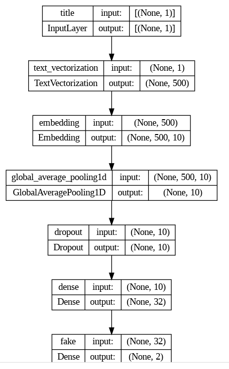
As we can see from the model graph, we have 7 layers. The first layer is input layer that accepts only title text. The second layer is embedding layer which turns a single word into 10 number vector whcih will later use to make a plot. We have two dense layers and a dropout layer to avoid overfitting. Next we optimize, define loss funcion and the metric to report so that we can decide which model to choose. Then we finally fit our model.
model_one.compile(optimizer="adam",
              loss = losses.SparseCategoricalCrossentropy(from_logits=True),
              metrics=["accuracy"])
history_one = model_one.fit(train,
validation_data=val,
epochs = 20,
verbose = True)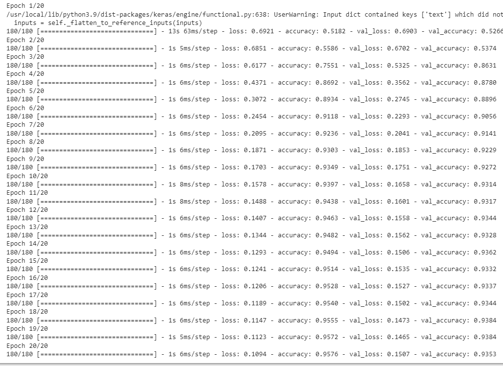
We then make a graph of training and accuracy scores. As we can see our model performs very well. There is no signs of overfitting or underfitting. The model’s accuracy score is around 93/%.
from matplotlib import pyplot as plt
plt.plot(history_one.history["accuracy"],label="train accuracy")
plt.plot(history_one.history["val_accuracy"],label="validation accuracy")
plt.title("Accuracy Scores for Different Epochs")
plt.xlabel("Epoch")
plt.ylabel("Accuracy")
plt.legend()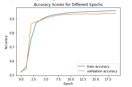
Model two
We follow the same process. The only difference is that instead of using title column as an input feature, we use text of the article as an input.
text_input = keras.Input(
    shape=(1,),
    name = "text",
    dtype = "string"
)

text_features = text_vectorize_layer(text_input)
text_features = layers.Embedding(size_vocabulary, output_dim=10, name='embedding')(text_features)
text_features = layers.GlobalAveragePooling1D()(text_features)
text_features = layers.Dropout(0.2)(text_features)
text_features = layers.Dense(32, activation='relu')(text_features)
output = layers.Dense(2, name="fake")(text_features)

model_two = keras.Model(
    inputs = text_input,
    outputs = output
)model_two.compile(optimizer="adam",
loss = losses.SparseCategoricalCrossentropy(from_logits=True),
metrics=["accuracy"])history_two = model_two.fit(train,
validation_data=val,
epochs = 20,
verbose = True)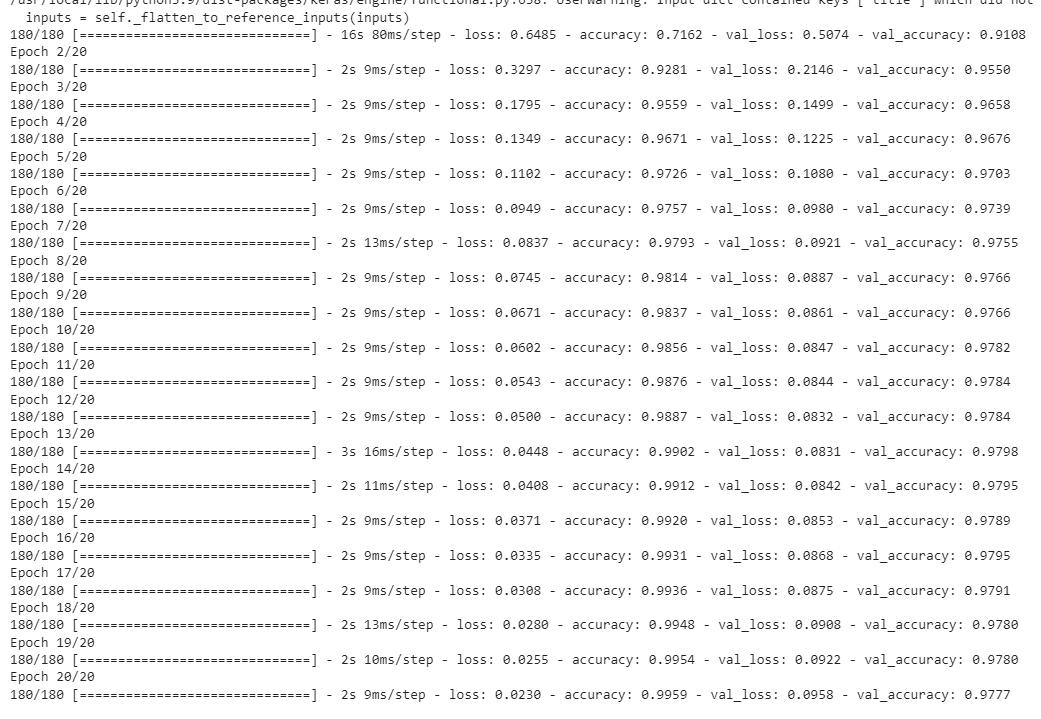
We then make a graph of training and accuracy scores. As we can see our model performs very well. There is no signs of overfitting or underfitting. The model’s accuracy score is around 97.8/% which is a significant improvement compared to model one.
from matplotlib import pyplot as plt
plt.plot(history_two.history["accuracy"],label="train accuracy")
plt.plot(history_two.history["val_accuracy"],label="validation accuracy")
plt.title("Accuracy Scores for Different Epochs")
plt.xlabel("Epoch")
plt.ylabel("Accuracy")
plt.legend()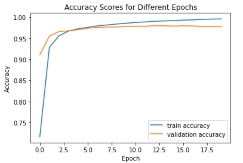
Model three
For this model we use both inputs - text and title data. We add this two branches by using concatenate layer.
text_features = text_vectorize_layer(text_input)
title_features = title_vectorize_layer(title_input)

main = layers.concatenate([text_features, title_features], axis = 1)

main = layers.Embedding(size_vocabulary, output_dim=10, name='embedding')(main)
main = layers.GlobalAveragePooling1D()(main)
main = layers.Dropout(0.2)(main)
main = layers.Dense(32, activation='relu')(main)
output = layers.Dense(2, name="fake")(main)

model_three = keras.Model(
    inputs = [text_input, title_input],
    outputs = output
)

model_three.compile(optimizer="adam",
              loss = losses.SparseCategoricalCrossentropy(from_logits=True),
              metrics=["accuracy"])

history_three = model_three.fit(train,
                    validation_data=val,
                    epochs = 20,
                    verbose = True)
We then make a graph of training and accuracy scores. As we can see our model performs very well. There is no signs of overfitting or underfitting. The model’s accuracy score is around 97.8/% which is a significant improvement compared to model one and it performs roughly equaivalently to model two.
from matplotlib import pyplot as plt
plt.plot(history_three.history["accuracy"],label="train accuracy")
plt.plot(history_three.history["val_accuracy"],label="validation accuracy")
plt.title("Accuracy Scores for Different Epochs")
plt.xlabel("Epoch")
plt.ylabel("Accuracy")

plt.legend()
Model Evaluation
After training our models, it is time to evaluate them on unseen data and see how our models perform. First we get the test data, prepocess it by passing it to make_dataset(), and evaluate all three models.
test_url = "https://github.com/PhilChodrow/PIC16b/blob/master/datasets/fake_news_test.csv?raw=true"
df_test = pd.read_csv(train_url)

dataset_test = make_dataset(df_test)

_ , test_accuracy_one = model_one.evaluate(dataset_test)
print('Test accuracy for model one:', test_accuracy_one)

_ , test_accuracy_two = model_two.evaluate(dataset_test)
print('Test accuracy for model two:', test_accuracy_two)

_ , test_accuracy_three = model_three.evaluate(dataset_test)
print('Test accuracy for model three:', test_accuracy_three)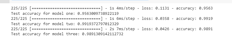
As we can see all three models perform really well. Model two and three perform slightly better than model one as expected. I chose model two as the final model. If we use my model as a fake news detector, it will make correct predictions 99 out of 100 times.
Visualization
In order to create two dimensional visualization we reduce the number of features by using PCA technique which reduces the number of features by keeping the variance as large as possible.
weights = model_two.get_layer('embedding').get_weights()[0] # get the weights from the embedding layer
vocab = text_vectorize_layer.get_vocabulary()                # get the vocabulary from our data prep for later

from sklearn.decomposition import PCA
pca = PCA(n_components=2)
weights = pca.fit_transform(weights)

embedding_df = pd.DataFrame({
    'word' : vocab,
    'x0'   : weights[:,0],
    'x1'   : weights[:,1]
})
import plotly.express as px
fig = px.scatter(embedding_df,
x = "x0",
y = "x1",
size = [2]*len(embedding_df),
hover_name = "word")
fig.show()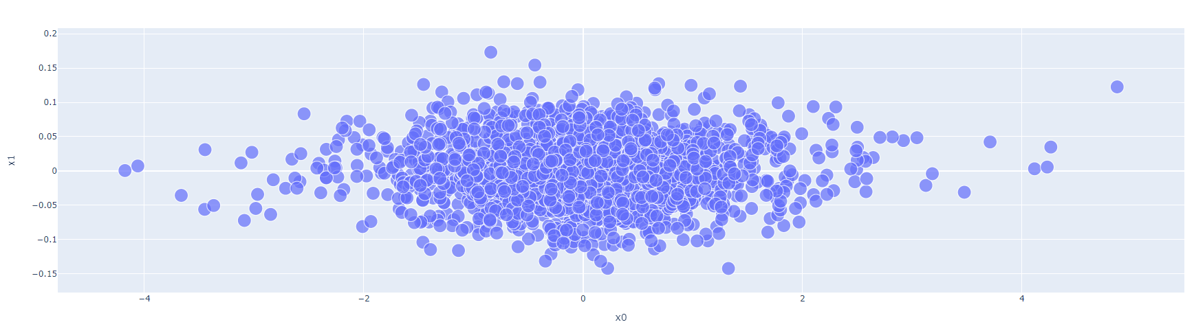
The left side seems to contain words that express strong feelings such as terror, radical, controversial, reportedly, and obvious. This might be an indicator that a news article is fake. On the other hand, the right side of the plot has words such as reporters, citing, and geographic names which might be an indicator of factual news.