Introduction

In this blog, we will build four models that classify dogs and cats photos with each previous model building on top of the other one. The last model uses a pre-trained model as a starting point for our cats and dogs classification model. Instead of training a new model from scratch as we did in the first three models, this model uses the knowledge learned by an existing model that has been trained on a larger dataset and does a pretty good job for image classification. We will see that some models overfit to the training dataset and learn a way to avoid overfitting. Finally, we will see how easy transfer learning makes training a model with high accuracy with very few parameters compared to the other models.

You can also access the code in the google colab format in this link: https://colab.research.google.com/drive/1jOBEvBFlkykrfxPHaOCHife_Xq6k3jwS#scrollTo=gpcZ8x0RykP9
Since showing the histories of the model training takes up a big space, the values of the histories shown in this blog are screencaps. The actual results can be viewed in the colab link provided above.

Obtaining Data

We start by making some imports.

import os
import tensorflow as tf
from tensorflow.keras import utils
from matplotlib import pyplot as plt
from tensorflow.keras import models, layers
import numpy as np

Next block of code enables us to access the data.

# location of data
_URL = 'https://storage.googleapis.com/mledu-datasets/cats_and_dogs_filtered.zip'

# download the data and extract it
path_to_zip = utils.get_file('cats_and_dogs.zip', origin=_URL, extract=True)

# construct paths
PATH = os.path.join(os.path.dirname(path_to_zip), 'cats_and_dogs_filtered')

train_dir = os.path.join(PATH, 'train')
validation_dir = os.path.join(PATH, 'validation')

# parameters for datasets
BATCH_SIZE = 32
IMG_SIZE = (160, 160)

# construct train and validation datasets 
train_dataset = utils.image_dataset_from_directory(train_dir,
                                                   shuffle=True,
                                                   batch_size=BATCH_SIZE,
                                                   image_size=IMG_SIZE)

validation_dataset = utils.image_dataset_from_directory(validation_dir,
                                                        shuffle=True,
                                                        batch_size=BATCH_SIZE,
                                                        image_size=IMG_SIZE)

# construct the test dataset by taking every 5th observation out of the validation dataset
val_batches = tf.data.experimental.cardinality(validation_dataset)
test_dataset = validation_dataset.take(val_batches // 5)
validation_dataset = validation_dataset.skip(val_batches // 5)

Found 2000 files belonging to 2 classes.

Found 1000 files belonging to 2 classes.

After running this block of code, we created a TensorFlow Dataset for training, validation, and testing. We use image_dataset_from_directory() function from utils library in keras to make these three datasets. This function has some arguments:
1. location of the images.
2. shuffle is set to True which means that the order of data when retrieved is randomized.
3. batch_size is set to 32 which means that 32 data points will be processed by our model at once.
4. image_size is set to (160, 160) in order to have a consistent image size.

This next code of block is technical related to the speed of reading the data.

AUTOTUNE = tf.data.AUTOTUNE

train_dataset = train_dataset.prefetch(buffer_size=AUTOTUNE)
validation_dataset = validation_dataset.prefetch(buffer_size=AUTOTUNE)
test_dataset = test_dataset.prefetch(buffer_size=AUTOTUNE)

Next let’s explore what our data consists of. This next function creates a two-row visualization of cats and dogs images. The first row contains all dog images and the second row contains cats.

from matplotlib import pyplot as plt

def two_row_visualization():
  """
  This function returns photos of cats and dogs.
  The photos of cats are returned on the first row 
  while the photos of dogs are returned on the second row.
  """
  plt.figure(figsize=(6,10))
  ax = plt.subplots(2,3)
  i = 0
  i_dog = 0
  i_cat = 3
  for images, labels in train_dataset.take(1):
    for i in range(len(labels)):
      if labels[i] == 1 and i_dog < 3:
        ax = plt.subplot(2, 3, i_dog + 1)
        plt.imshow(images[i].numpy().astype("uint8"))
        plt.title('dog')
        plt.axis("off")
        i_dog += 1
        i += 1
      elif labels[i] == 0 and i_cat < 6:
        ax = plt.subplot(2, 3, i_cat + 1)
        plt.imshow(images[i].numpy().astype("uint8"))
        plt.title('cat')
        plt.axis("off")
        i_cat += 1
        i += 1
      elif i_dog == 3 and i_cat == 6:
        break

In order to access a piece of data in the training dataset, we use train_dataset.take(1) function which randomly retrieves one batch of data from the train_dataset. two_row_visualization() function creates a 2 by 3 figure with dog photos on the first row (cause they are better) and cat photos on the second row. Let’s run this function and see how it works.

two_row_visualization()

<Figure size 576x960 with 0 Axes>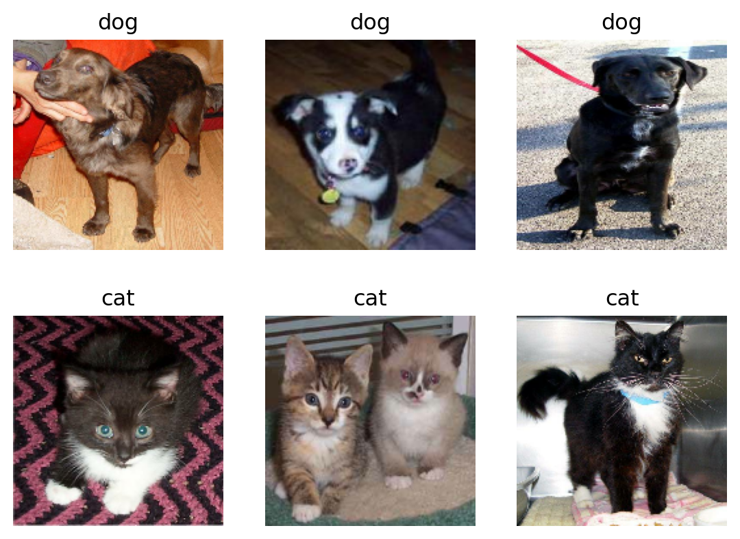

This block computes the number of cat and dog images in the training data set.

labels_iterator= train_dataset.unbatch().map(lambda image, label: label).as_numpy_iterator()
cat = 0
dog = 0

for i in labels_iterator:
  if i == 0:
    cat += 1
  else:
    dog += 1

print(f"There are {cat} cats and {dog} dogs in the training dataset.")

There are 1000 cats and 1000 dogs in the training dataset.

The first line of code creates an iterator of labels. The rest of the code is a for loop that counts the number of cat and dog images.

As we see our model has an equal number of training samples for both cats and dogs. If we use the baseline machine learning model, i.e. the model that always guesses the most frequent label, it will always either guess cats or dogs. Therefore the accuracy of the baseline model is 50 percent.

Model One

Now let’s move to the exciting part of this blog - creating models.

from tensorflow.keras import models, layers

tf.random.set_seed(0)

model1 = models.Sequential([
    layers.Conv2D(32, (3,3)),
    layers.MaxPooling2D((2,2)),
    layers.BatchNormalization(),
    layers.Activation("relu"),
    layers.Conv2D(64, (3,3), activation='relu'),
    layers.MaxPooling2D((2,2)),
    layers.Conv2D(64, (3,3), activation='relu'),
    layers.MaxPooling2D((2,2)),
    layers.Flatten(),

    layers.Dense(128, activation='relu'),
    layers.Dropout(.5),
    layers.Dense(2)
])

This model is made up of 3 Conv2D layers with 32, 64, 64 output channels. Each Conv2D is followed by a MaxPooling2D layer which reduces the size of the image by replacing with the maximum each 2 by 2 square block of the image. The Flatten layer turns a multidimensional (in this case 3D) input into a 1D array. We have one Dense layer which takes this 1D flattened array and produces 128 outputs. Some of these layers have an activation function which is the nonlinear function that we apply to the output of the neurons. In this case we choose to use the Relu function which is defined as \(f(x)=max(x,0)\). Next we apply Dropout layer with 0.5 rate. This randomly freezes half of the units of the previous layer in each iteration. This serves as a way to avoid overfitting by forcing the algorithm to find different paths rather than relying heavily on a single path. The last Dense layer has 2 outputs which are expected as the number of outputs should be 2 - cats or dogs.

Next we compile the model. This initializes the optimizer. Optimizer is an algorithm that is used to update the weights and biases of the network during training in order to minimize the loss function. It initializes loss function which is set to categorical cross entropy. It measures the difference between the predicted probability distribution and the true label distribution. Finally, we set the metric to be accuracy which we will use to evaluate the model.

model1.compile(optimizer='adam', 
              loss = tf.keras.losses.SparseCategoricalCrossentropy(from_logits=True),
              metrics = ['accuracy'])

Now let’s fit the model and see how it performs.

history1 = model1.fit(train_dataset, 
                     epochs=20, 
                     validation_data=validation_dataset,
                     verbose=0)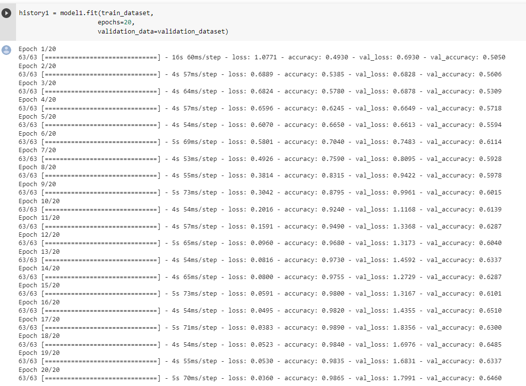

The validation accuracy of this model stabilizes between 62% and 65% during the training. By comparing this to the basline model which has an accuracy score of 50% we see some improvement. As we can see the training accuracy score is significantly bigger (it is more than 90%) than the validation accuarcy score which means that our data overfits badly.

Model two

In this model we use data augmentation to avoid overfitting to the training data. We use RandomFlip and RandomRotation layers to make random flips and rotations of the photos. Since the photo of a cat or dog is still a photo of a cat of a dog even if it is fliped or rotated, we benfit from this as now our model is not prone to overfit. Let’s see how these layers work on this photo.

for image, label in train_dataset.take(1):
  random_image = image[0]
  break

plt.imshow(random_image.numpy().astype("uint8"))
plt.axis("off")

(-0.5, 159.5, 159.5, -0.5)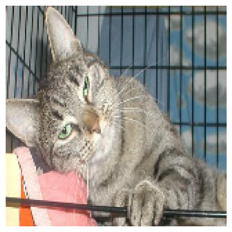

We first apply horizontal and vertical flip on the photo.

plt.figure(figsize=(6,10))
ax = plt.subplots(2,3)
flip_layer = tf.keras.layers.RandomFlip( mode="horizontal_and_vertical", seed=0)
for i in range(6):
  ax = plt.subplot(2, 3, i + 1)
  plt.imshow(flip_layer(random_image).numpy().astype("uint8"))
  plt.axis("off")

<Figure size 576x960 with 0 Axes>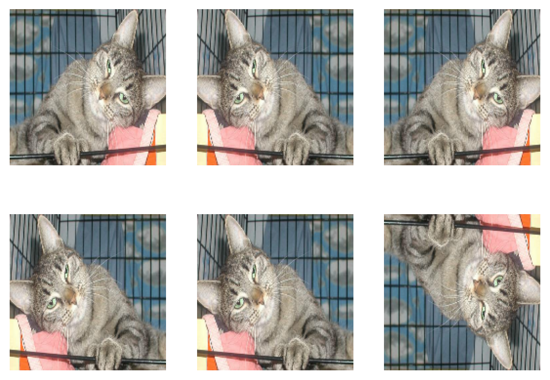

Now let’s see what the photos look like when we apply RandomRotation function with factor 0.2. It flips the photos 0.2*2pi either clockwise or counter-clockwise.

plt.figure(figsize=(6,10))
ax = plt.subplots(2,3)
flip_layer = tf.keras.layers.RandomRotation(factor=0.2, seed=0)
for i in range(6):
  ax = plt.subplot(2, 3, i + 1)
  plt.imshow(flip_layer(random_image).numpy().astype("uint8"))
  plt.axis("off")

<Figure size 576x960 with 0 Axes>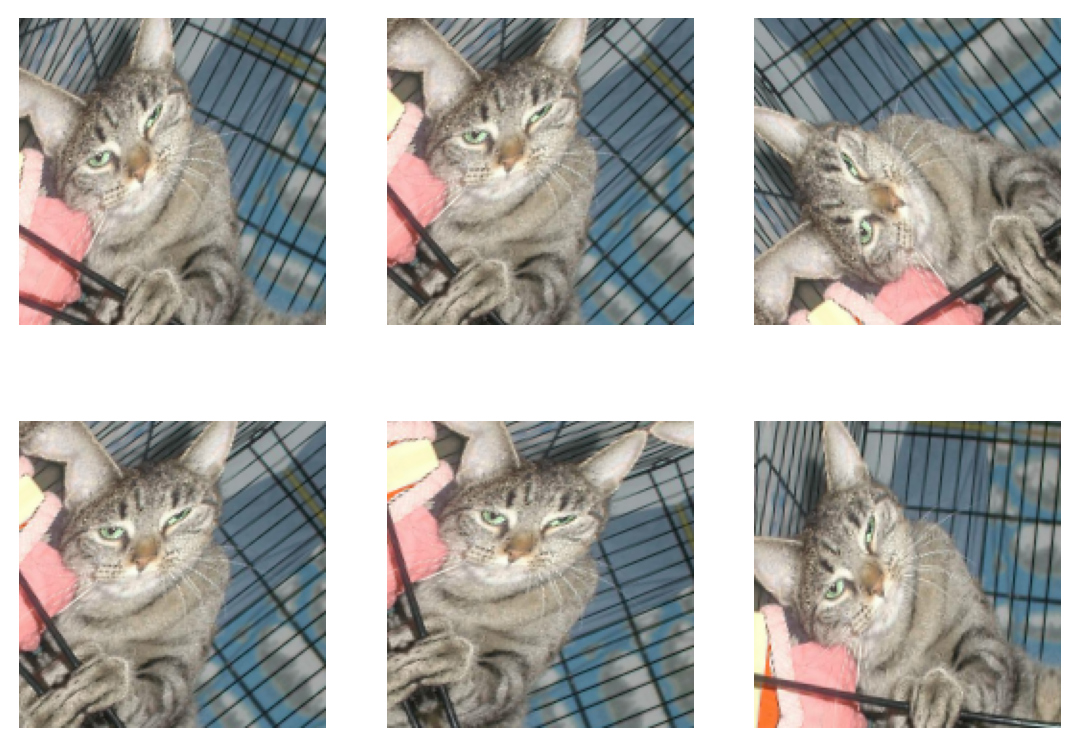

We add these two layers to our first model and call this new model model2.

model2 = models.Sequential([
    tf.keras.layers.RandomFlip( mode="horizontal_and_vertical", seed=0),
    tf.keras.layers.RandomRotation(factor=0.2, seed=0),
    layers.Conv2D(32, (3,3)),
    layers.MaxPooling2D((2,2)),
    layers.BatchNormalization(),
    layers.Activation("relu"),
    layers.Conv2D(64, (3,3)),
    layers.MaxPooling2D((2,2)),
    layers.BatchNormalization(),
    layers.Activation("relu"),
    layers.Conv2D(64, (3,3)),
    layers.MaxPooling2D((2,2)),
    layers.BatchNormalization(),
    layers.Activation("relu"),
    layers.Flatten(),

    layers.Dense(128, activation='relu'),
    layers.Dropout(.5),
    layers.Dense(2)
])

Again we compile the model and fit to our training dataset.

model2.compile(optimizer='adam', 
              loss = tf.keras.losses.SparseCategoricalCrossentropy(from_logits=True),
              metrics = ['accuracy'])

history2 = model2.fit(train_dataset, 
                     epochs=30, 
                     validation_data=validation_dataset)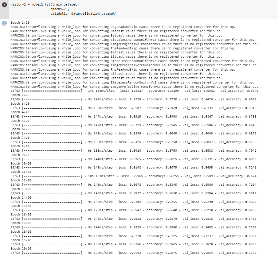

The validation accuracy of this model stabilizes between 56% and 72% during the training. By comparing this to model one, we see that model two performs a little better but the stabilization region is larger. This might be caused by random flipping and rotation introduced in this model. As we can see the training accuracy score is in the same range as the validation accuracy score which means that our data does not overfit anymore.

Model three

In this model we introduce a new layer that normalizes the data for color channels. Instead of having RGB values that range between 0 and 255 we normalize them. This speeds up the weight assignment since the weights don’t need to scale up for the bigger range which saves a lot of unnecessary computations and speeds up the training process.

i = tf.keras.Input(shape=(160, 160, 3))
x = tf.keras.applications.mobilenet_v2.preprocess_input(i)
preprocessor = tf.keras.Model(inputs = [i], outputs = [x])

model3 = models.Sequential([
    preprocessor,
    tf.keras.layers.RandomFlip( mode="horizontal_and_vertical", seed=0),
    tf.keras.layers.RandomRotation(factor=0.2, seed=0),
    layers.Conv2D(32, (3,3)),
    layers.MaxPooling2D((2,2)),
    layers.BatchNormalization(),
    layers.Activation("relu"),
    layers.Conv2D(64, (3,3)),
    layers.MaxPooling2D((2,2)),
    layers.BatchNormalization(),
    layers.Activation("relu"),
    layers.Conv2D(64, (3,3)),
    layers.MaxPooling2D((2,2)),
    layers.BatchNormalization(),
    layers.Activation("relu"),
    layers.Flatten(),

    layers.Dense(128, activation='relu'),
    layers.Dropout(.5),
    layers.Dense(2)
])

model3.compile(optimizer='adam', 
              loss = tf.keras.losses.SparseCategoricalCrossentropy(from_logits=True),
              metrics = ['accuracy'])

history3 = model3.fit(train_dataset, 
                     epochs=20, 
                     validation_data=validation_dataset)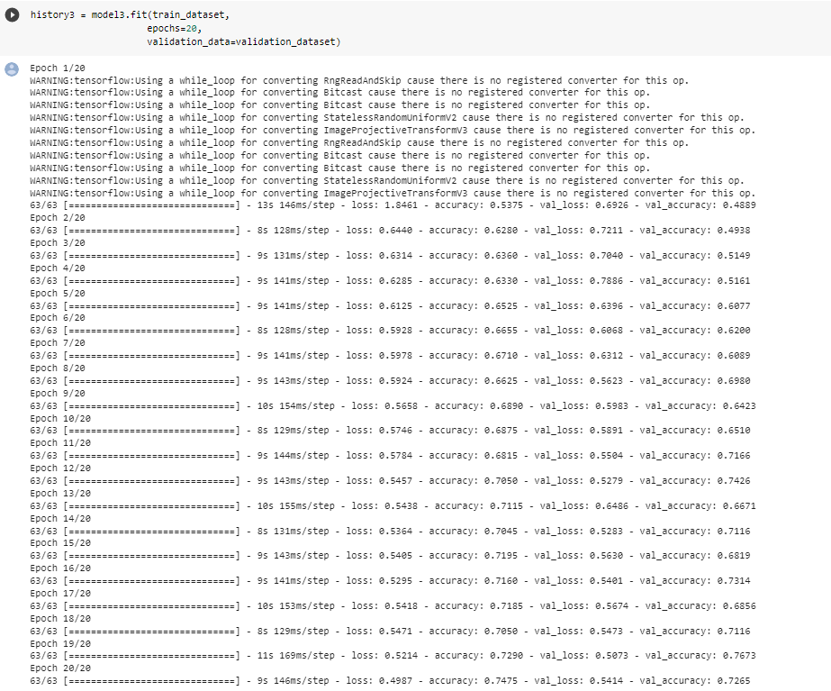

The validation accuracy of this model stabilizes between 68% and 74% during the training. By comparing this model to model one, we see that model three performs much better. This improvement is due to the normalization of color channels which enabled the algorithm to find valuable connections in the neural network instead of wasting a lot of time to adjust weights for larger scales of RGB values. As we can see the training accuracy score is in the same range as the validation accuracy score which means that our model does not overfit.

Model four

In this model we use a technique called transfer learning. The idea is to incorporate a pre-trained model (“base model”) into our model as a starting point instead of starting from scratch. Our model performs better as pre-trained models are usually trained on a large dataset, and has learned to recognize a wide range of features that are often useful.

IMG_SHAPE = (160, 160) + (3,)
base_model = tf.keras.applications.MobileNetV2(input_shape=IMG_SHAPE,
                                               include_top=False,
                                               weights='imagenet')
base_model.trainable = False

i = tf.keras.Input(shape=IMG_SHAPE)
x = base_model(i, training = False)
base_model_layer = tf.keras.Model(inputs = [i], outputs = [x])

model4 = models.Sequential([
    preprocessor,
    tf.keras.layers.RandomFlip( mode="horizontal_and_vertical", seed=0),
    base_model_layer,
    tf.keras.layers.RandomRotation(factor=0.2, seed=0),
    layers.Conv2D(32, (3,3), padding='same'),
    layers.MaxPooling2D((2,2)),
    layers.BatchNormalization(),
    layers.Activation("relu"),
    layers.Conv2D(64, (3,3), padding='same'),
    layers.MaxPooling2D((2,2)),
    layers.BatchNormalization(),
    layers.Activation("relu"),
    layers.Flatten(),

    layers.Dense(32, activation='relu'),
    layers.Dropout(.5),
    layers.Dense(2)
])

model4.compile(optimizer='adam', 
              loss = tf.keras.losses.SparseCategoricalCrossentropy(from_logits=True),
              metrics = ['accuracy'])

history4 = model4.fit(train_dataset, 
                     epochs=10, 
                     validation_data=validation_dataset)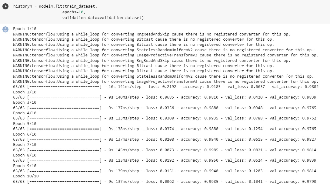

As we can see this model performs the best. We don’t need many epochs to get the desired accuracy score. This model’s validation score stabilizes between 97% and 98.5%. The accuracy score is the best compared to all the previous models that were all trained from scratch. The base model indeed improved the performance of our model. In this case we see some overfitting as the model achieves 99% accuracy on training data. Also we can see from validation and training accuracy score and loss below that we have overfitting.

acc = history4.history['accuracy']
val_acc = history4.history['val_accuracy']

loss = history4.history['loss']
val_loss = history4.history['val_loss']

epochs_range = range(1,11)

plt.figure(figsize=(8, 8))
plt.subplot(1, 2, 1)
plt.plot(epochs_range, acc, label='Training Accuracy')
plt.plot(epochs_range, val_acc, label='Validation Accuracy')
plt.legend(loc='lower right')
plt.title('Training and Validation Accuracy')

plt.subplot(1, 2, 2)
plt.plot(epochs_range, loss, label='Training Loss')
plt.plot(epochs_range, val_loss, label='Validation Loss')
plt.legend(loc='upper right')
plt.title('Training and Validation Loss')
plt.show()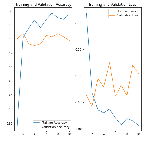

Score on Test Data

Finally let’s evaluate our last model (best performing model) on unseen test data.

loss, accuracy = model4.evaluate(test_dataset)
print('Test loss:', loss)
print('Test accuracy:', accuracy)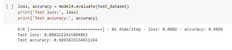

The results are around 99%. Hurray! The model performs very well.